Catenary Calculator (Point Load)
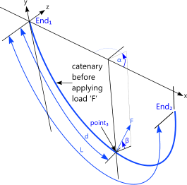
Fig 1. Catenary Before Applying 'F'
Please refer to CalQlata's Catenary technical help page for a detailed description of the properties of a catenary.
A single catenary always occupies a single vertical plane (it hangs vertically down) as its shape is created by the force of gravity (Fig 1).
If you pick it up or pull it down at any point (3) along its length, which we will refer to as point₃, with a point-load (or force 'F') you will automatically generate two independent catenaries joined at point₃ (Figs 2, 3 & 4). The fact that these catenaries are both independent means that the distribution of 'F' between them is not self-evident (it is not shared equally in any direction).
Therefore the impact of 'F' on each original end support (End₁ and End₂) will vary according to the relevant distances from either end, i.e. the orientation of application and horizontal tension in the original catenary.
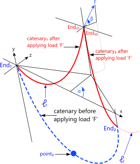
Fig 2. Catenary After Applying 'F'
Depending upon the configuration you are trying to achieve and the pull-direction or location (along the catenary) available, you may need to perform a number of calculations in order to discover the optimum location of Point₃ along with the magnitude and/or orientation of your force to achieve the desired result.
Iterative Calculation
This catenary calculator uses a multiple 'nested' iteration procedure that synchronises all forces and dimensions to within pre-defined error levels; such that; ε<5.0E-09.
Should you apply extreme conditions to your catenary before applying 'F': e.g. setting 'x' to less than 1% of its length can sometimes generate errors⁽¹⁾.
Owing to the hyperbolic/exponential nature of catenary formulas, 'bar-tight' configurations may also increase iteration errors. As such, applying a force of e.g. twice the mass of the catenary to a point less than 5% along its length from either end is not recommended as a means of achieving best results.
For the same reason, when applying loads at the limits of the calculator's capabilities (bar-tight, tiny or excessive loads, outside the aforementioned ±5% area), you may find that applied-angles (α & β) close to 0°, 90° and 180°# may result in errors. In such cases, you may need to modify the applied angle and/or applied load to achieve a result.
# Angles at or close to 0°, 90° and 180° have not been approximated in this calculator to avoid lack of accuracy (>ε) in normal calculations.
The error "whoops! not possible" only applies to a loaded catenary. The unloaded catenary calculation results are correct even if this error message appears.
Catenary+ Calculator - Technical Help
Units
You may use any units you like, but you must be consistent.
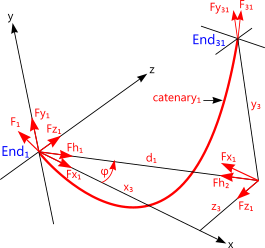
Fig 3. Forces on Catenary₁ Supports
Calculation Setup
This catenary calculator has been designed to apply a point-load to a predefined (unloaded) catenary. Accordingly, when first loading Catenary+ you will need to generate an unloaded catenary.
The unloaded catenary requires the following input data: x₂, y₂, L and w;
inputs d and p are required only for the properties at any point along its length.
The remaining input data; F (>0), α (1≤179) and β (-89.95<89.95) are required to define the mid-length applied load.
Whilst the images generated by Catenary+ are not true catenaries, (they are corrected to show the shapes projected when seen from Plan, Front or Side elevations i.e. Perpendicular to x,z x,y or y,z planes respectively), the co-ordinates provided in the Data Listing window (immediately below the output data) for the two resultant catenaries (catenary₁ and catenary₂) are for 'True' configurations, i.e. as seen from a position perpendicular to the plane of each catenary⁽⁴⁾.
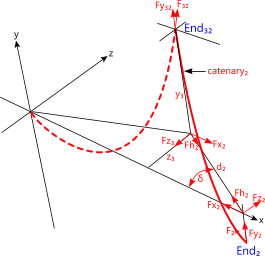
Fig 4. Forces on Catenary₂ Supports
The plots generated in this calculator are divided into 100 co-ordinate segments⁽²⁾.
Plot co-ordinates are provided in Catenary+ (menu item: 'Data Listing>Plot Co-ordinates') for a number of reasons:
1) generating plot images of the true catenary as opposed to those generated within the calculator, which are parallel with the co-ordinate planes
2) post-processing the co-ordinate data
3) plotting angles (θ) or lengths (l) with co-ordinates (x,y)
4) incorporation into other software
5) your operating system software may not cope with Catenary+'s graphical code, albeit this should not be the case with Windows-based software
Independent Checking Procedure
Owing to the complex nature of this calculation, it is always wise to carry out independent verification of a program's calculations in order to generate confidence in its output data. CalQlata has listed below a worked example using a combination of hand calculations and our other calculators to verify Catenary+
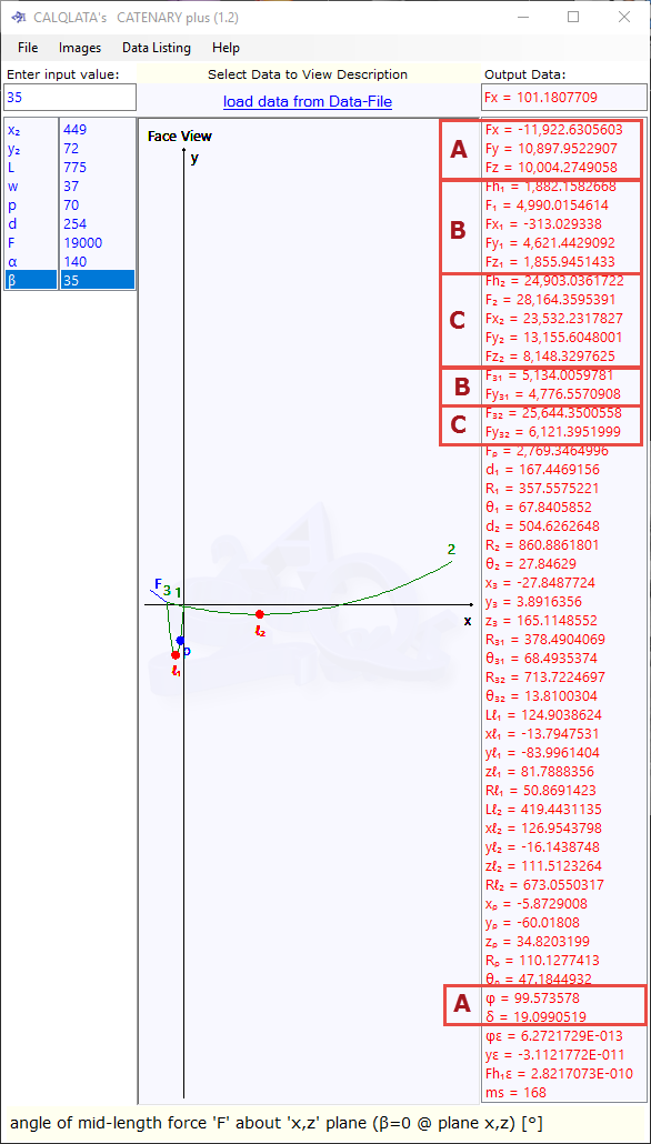
Step 1. Check the resolution of 'F' into its three dimensional axis forces by hand as follows:
Fh = F x Cos(β) (15,563.9 = 19,000 x Cos(35°))
Fx = Fh x Cos(α) (-11,922.6 = 15,563.9 x Sin(140°))
Fy = F x Sin(β) (10,897.95 = 19,000 x Sin(35°))
Fz = Fh x Sin(α) (10,004.27 = 15,563.9 x Sin(140°))
'Fx', 'Fy' and 'Fz' of which can be checked in Fig 5(A)
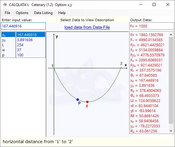
Step 2. Transfer data for catenary₁ from Catenary+ to the Catenary calculator (or check by hand calculation if you prefer). The data you will need from Catenary+ is provided in the results as follows (Figs 5(B) & Fig 6):
'L' (Catenary) = 'd' (Catenary+)#
{254}
'w' (Catenary) = 'w' (Catenary+)#
{37}
'x₂' (Catenary) = 'd₁' (Catenary+)#
{167.446916}
'y₂' (Catenary) = 'y₃' (Catenary+)#
{3.8916356}
(Or
'Fx' (Catenary) = 'Fh₁' (Catenary+)
{1882.1582768}
'Fy₂' (Catenary) = 'Fy₃₁' (Catenary+)
{4776.5570908}
Depending upon whether you prefer to use 'Catenary (x,y)' or 'Catenary Fx,Fy)' calculation options in Catenary.)
And compare the results:
'F₁' (Catenary) = 'F₁' (Catenary+)
{4990.015461}
'θ₁' (Catenary) = 'θ₁' (Catenary+)
{67.840585}
'Fy₁' (Catenary) = 'Fy₁' (Catenary+)
{4621.442902}
'F₂' (Catenary) = 'F₃₁' (Catenary+)
{5134.005988}
'θ₂' (Catenary) = 'θ₃₁' (Catenary+)
{68.493537}
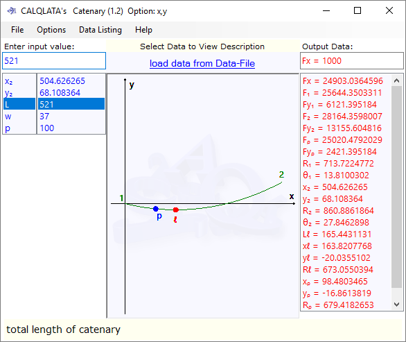
Step 3. Transfer data for catenary₂ from Catenary+ to the Catenary calculator (or check by hand calculation if you prefer). The data you will need from Catenary+ is provided in the results as follows (Figs 5(C) & Fig 7):
'L' (Catenary) = 'L' – 'd' (Catenary+)#
{521}
'w' (Catenary) = 'w' (Catenary+)#
{37}
'x₂' (Catenary) = 'd₂' (Catenary+)#
{504.626265}
'y₂' (Catenary) = 'y₃' - 'y₂' (Catenary+)#
{68.108364}
(Or
'Fx' (Catenary) = 'Fh₂' (Catenary+)
{24,903.036459 vs 24,903.036172}
'Fy₁' (Catenary) = 'Fy₃₂' (Catenary+)
{6,121.395184 vs 6,121.3952}
Depending upon whether you prefer to use Catenary (x,y) or Catenary Fx,Fy) calculation options in Catenary.)
And compare the results:
'F₂' (Catenary) = 'F₂' (Catenary+)
{28,164.359800 vs 28,164.359539}
'θ₁' (Catenary) = 'θ₃₂' (Catenary+)
{13.81003}
'Fy₂' (Catenary) = 'Fy₂' (Catenary+)
{13,155.604816 vs 13,155.6048}
'F₁' (Catenary) = 'F₃₂' (Catenary+)
{25,644.350331 vs 25,644.350056}
'θ₂' (Catenary) = 'θ₂' (Catenary+)
{27.84629}
Step 4. A plan view of the two resultant catenaries is always a triangle (Figs 2 & Fig 4) so hand calculation verification is simpler. You can use CalQlata's Trig calculator (Fig 8) or you can use the cosine rule provided in CalQlata's Trig technical help page and also in our 'Useful Stuff' page: Trigonometric Compound Formulas for a hand-calculation.
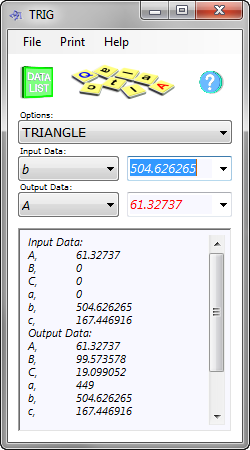
Fig 8. Trig Comparison for Plan View
As you already know δ and φ you can calculate the unknown angle (180 - δ - φ) which, in this case is: 61.32737° (180° – 19.099052° – 99.573578°). The angle 'A' (Fig 8) is subtended by sides: 'b' and 'c', which relate to 'd₂' and 'd₁' respectively. A correct calculation will show the length of side 'a' (opposite angle 'A') equal to 'x' in Catenary+ (449 in this case) and the two calculated angles 'B' & 'C' should equal φ and δ (99.573578 and 19.099052 respectively in this case).
Step 5: A similar approach may be used to check the axis-forces in Catenary+. For example:
'Fz' (10,004.274906) should be equal to 'Fz₁' + 'Fz₂' (1,855.945143 + 8,148.329763), which is correct.
'Fx₁' = Fh₁ x Cos(φ)
(1,882.158267 x Cos(99.573578°) = 313.029338)
'Fx₂' = Fh₂ x Cos(δ)
(24,903.036172 x Cos(19.099052°) = 23,532.231783)
Etc.
Accuracy
The above verification calculation is typical in that it produces the following errors:
'φε', 2.5868196E-013
'yε', -2.5147529E-010
'Fh₁ε', 2.8830982E-010
… few of which have manifested themselves in the above results comparison (between Catenary+, Trig and Catenary) and those that have, represent less than a millimetre in over ¾kilometer of catenary length, so may be considered irrelevant for all practical purposes.
Sign Convention
We have used a hybrid sign convention in order to maximise compatibility with our Catenary calculator. In general:
All forces are assumed positive according to the point load applied by the support onto the catenary at the end concerned (see Figs 3 & 4).
Notes
- The iteration speed of any normal calculation is practically instantaneous (about 150 milliseconds dependent upon the speed of your processor) and therefore not noticeable unless you are quickly typing a long number into the input data text-box in which case you might notice a slight delay.
- Refer to the Catenary technical help page 'Plotting your Curve' for instructions on how to generate spreadsheet plots using these co-ordinates.
Further Reading
You will find further reading on this subject in reference publications(3 & 9)

